Optimizing an OpenACC Weather Simulation Kernel

In this blog article I describe recent work to optimize an OpenACC code provided by the UK Met Office. This relatively small computational section has been developed as part of preparations to move to the new LFRic Weather Simulation Model. LFRic will be developed using an automated system called PSyclone which itself is currently under development at The Hartree Centre to generate performance-portable parallel code, including OpenACC-augmented Fortran for execution on GPUs. The hand-tuning of the code described in this blog provides a “gold standard” for PSyclone, to ensure that it is developed in a way that permits good performance on the GPU architecture.

The optimizations I describe are similar to those I have applied to many other types of scientific application in the past (for example, see a recording of my GTC18 talk), so many of the techniques are generally transferable. The results demonstrate the dramatic impact that relatively minor changes can have.

Original Code

First, let’s take a look at the original code, as it existed before any optimization. The purpose is to perform matrix-vector multiplications using custom formats. The outer body has the following structure:

do color = 1, ncolor
   !$acc parallel loop
   do cell = 1, ncp_color(color)
      …
      call matrix_vector_code(…)
   end do
end do

The GPU kernel is created from the code within the parallel loop syntax, which is within the outermost loop over ncolor , set to 6 in this example. Therefore, the resulting GPU kernel will be invoked 6 times. The loop over cell is mapped by the compiler to OpenACC gang-level parallelism (or - in CUDA terminology - block-level parallelism) on the GPU.  As can be seen, the functionality operating on each cell is not contained within this code unit but instead exists in a subroutine, matrix_vector_code (existing in a separate file), which is called by each thread. The original version of the subroutine contains the following code:

1  !$acc loop vector 
2  do k = 0, nlayers-1
3    lhs_e(:,:) = 0.0_r_def
4    ik = (cell-1)*nlayers + k + 1
5
6    do df = 1, ndf1
7      do df2 = 1, ndf2
8        lhs_e(df,k) = lhs_e(df,k) + matrix(df,df2,ik)*x(map2(df2)+k)
9   	end do
10   end do
11
12    do df = 1, ndf1
13      lhs(map1(df)+k) = lhs(map1(df)+k) + lhs_e(df,k)
14    end do
15
16  end do 

Performance Optimization

When running on the NVIDIA Tesla V100 GPU, the original code (compiled by the PGI compiler, which we use throughout) took 9.45ms. While this is only a fraction of a second, in a real simulation it would be repeated many, many times, and we will actually see there is plenty of room for improvement. This graph shows, left to right, the impact of several optimizations (each including the previous), to ultimately reduce the time by a factor of around 30X down to 0.32ms.

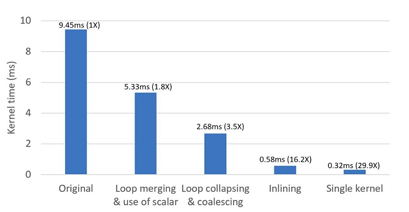
The optimizations involve the removal of unnecessary memory accesses; the restructuring and collapsing of loops to get better parallelism mapping and memory access patterns; the inlining of a subroutine to reduce register pressure; and the combination (i.e. fusion) of multiple kernels. In the next sections, we will look at these optimizations in more detail.

Loop merging and replacement of array with scalar

The first notable point is that if we merge the two loops over df (lines 6 and 12), that allows us to replace the lhs_e temporary array structure with a scalar, as follows:

do df = 1, ndf1
   lhs_e_scal=0.0_r_def 
   do df2 = 1, ndf2
      lhs_e_scal = lhs_e_scal + matrix(df,df2,ik)*x(map2(df2)+k)
   end do

   lhs(map1(df)+k) = lhs(map1(df)+k) + lhs_e_scal
end do

This scalar can then remain resident in a register (for each GPU thread), and we avoid unnecessary memory accesses. While this nearly doubles the performance, at this stage we have not fully exposed the available parallelism, and our memory access patterns remain suboptimal.

Loop Collapsing and Memory Coalescing

The OpenACC directive at line 1 has the effect of mapping the outermost loop (over k) to vector-level parallelism: in CUDA programming model terms, each CUDA thread will operate on a separate value of k, and will loop over df (and df2 ). However, the loop over df is also data-parallel, and we can choose to expose that parallelism also at the vector level:

!$acc loop vector collapse(2)
   do k = 0, nlayers-1
      do df = 1, ndf1
      ...

The collapse(2) clause has the effect of transforming the subsequent two loops into a single loop, and mapping the resulting combined loop to the vector (CUDA thread) level. This not only increases the extent of parallelism exposed to our hardware, but also allows memory coalescing into the matrix. GPUs offer very high bandwidth to global memory (relative to CPUs), but the achieved throughput depends on the access patterns occurring in the application: to get good performance it is necessary that neighbouring parallel threads access neighbouring memory locations, such that the multiple threads cooperate to load coalesced chunks of data. For more information on memory coalescing I suggest watching this presentation recording.

In this case, the matrix array has df as its fastest moving index, so consecutive df values correspond to consecutive memory locations. Therefore, for memory coalescing we also require consecutive CUDA threads to correspond to consecutive df values. This is now achieved, because the loop over df is the innermost loop in the collapsed nest.

Note that we now require the update of lhs (line 13) to be atomic since multiple df values may map to the same map1(df) index. Therefore we introduce !$acc atomic update above this line.

Note also that memory accesses into the vector x are not coalesced since these have k as the fastest moving array index. However, this is not so important since the same x elements are re-used for multiple df elements, so the values are shared across multiple threads within a vector, and between multiple vectors through caching. Nevertheless it is possible to achieve full coalescing by using a transposed format for the matrix which has ik as the fastest moving index, and also interchanging the order of the two collapsed loops such that the loop over k is innermost. We tried this but did not observe any significant advantage.

Our final subroutine is as follows

!$acc loop vector collapse(2)
   do k = 0, nlayers-1
      do df = 1, ndf1

         ik = (cell-1)*nlayers + k + 1
         lhs_e_scal = 0.0_r_def

         do df2 = 1, ndf2
            lhs_e_scal = lhs_e_scal + matrix(df,df2,ik)*x(map2(df2)+k)
         end do
      
         !$acc atomic update
         lhs(map1(df)+k) = lhs(map1(df)+k) + lhs_e_scal

   end do
end do

We find that this performs much better than the previous versions, but is still not optimal because it has large register usage resulting in low occupancy of the GPU.

Reducing register usage through inlining

The register usage can be reduced by the compiler if the subroutine can be inlined into the main body of the kernel. Since the subroutine exists in a different file from the main body of the kernel, we can leverage the Inter Procedural Analysis (IPA) functionality of the PGI compiler to perform such inlining. We include the -Mipa=inline:reshape -Minfo flags at the compilation and linking stages (which instruct the compiler to perform IPA even when array shapes don’t match, and provide information on the transformations applied, respectively), and we see output such as 69, matrix_vector_code inlined, size=24 (IPA) file matrix_vector_kernel_mod.F90 (68) which confirms inlining has been successful.

Combining Multiple Colors into a Single Kernel

Looking back at the original outer-body of the kernel, we see that multiple kernels are launched corresponding to multiple “colors”. Such a structure is common where there exist dependencies which enforce serialization, but in this case no such dependencies exist and we can fully expose parallelism by combining into a single kernel. We do this in the following way:

!$acc parallel loop collapse(2) …
do color = 1, ncolor
   do cell = 1, ncp_color_max
      if (cell .lt. ncp_color(color)) then
         …

As shown, we move the OpenACC parallel loop directive to the outermost level, and use the collapse(2)  clause to specify that the two loops should be collapsed and the resulting loop should be mapped to gang (CUDA block of threads) level parallelism. Note that, to allow the compiler to parallelize, we remove the dependence of the inner loop extent on the outer loop index (ncp_color(color))  by replacing this with a pre-computed max value ncp_color_max and introducing an if statement to mask out the unwanted iterations. Therefore, the resulting kernel will have some thread-blocks which do nothing, but the nature of CUDA’s highly-parallel block scheduling philosophy means that these thread-blocks with immediately exit and hence this does not have a detrimental effect on performance. With a single kernel, we are now exposing far more parallelism to the GPU within a single invocation, we avoid multiple launch overheads, and we provide better opportunities to cache any re-used data on-chip.

But How Good is it Now?

It is important to understand the performance of our final optimized version in relation to that expected from the hardware in use, to ascertain if we have any scope for further improvement. We can use the NVIDIA Profiler to obtain metrics which help us towards this goal:

The combination of the results of the dram_read_throughput and dram_write_throughput metrics give us the overall achieved throughput to the off-chip HBM2 memory on the V100, and flop_count_dp gives us the number of double precision floating point operations executed. In the spirit of a roofline model analysis, we can combine these (together with the kernel time) to get the Arithmetic Intensity (ratio of flops per byte) to get 0.3 flops/byte: very low compared to the ridge point for the hardware (9.9 flops/byte). Therefore, we know that the code is memory bandwidth bound (and not compute bound). We then compare our memory throughput, 549 GB/s, to the value obtained using the industry-standard STREAM benchmark, and we find that our kernels are achieving around 70% of STREAM throughput, which indicates that the code is reasonably well-optimized for a real application kernel. It is possible that further optimizations may exist to increase this performance more, but it is arguably now at an acceptable level taking into account the trade-off between code maintainability and in-depth optimizations.